How to combine RADEX and MCMC

RADEX (van der Tak et al. 2007) is a simple but powerful code to solve non-LTE radiative transfer, and has been widely used in various astronomical environments. Generally, we use this code to fit the physical parameters of a molecular cloud with multiple transitions of a single molecular species. When fitting the data, we tend to minimize a loss function (or something similar), and MCMC (Markov chain Monte Carlo) is a powerful method to get the global minimum (instead of local minimum, which is the drawback of other methods like scipy.optimize.curve_fit whose fitting results strongly depend on the initial values given by the user) and a robust estimation of the error.

I am a heavy user of RADEX, but know little about MCMC. However, it seems that we can still run a basic MCMC fitting code without a rich knowledge about how MCMC works. It is never a bad choice, though, to know more about MCMC before you start using it. This blog mainly refers to the basic tutorial of emcee, the radex_emcee code written by Chentao Yang, and my private conversation with my roomate. I do not guarantee that everything in this blog is correct.

Prerequisites

The following codes are run in Jupyter Notebook. Other packages you may need are:

• emcee to run MCMC and corner to make corner plots.
• a python interface of RADEX. I choose spectralradex (Note that you must not use pandas>2.0 with spectralradex. See this issue for details. Also note that spectralradex can only work when the number of lines is <500, otherwise you need to modify the code following this), and myRadex is also a good choice. You can also write a simple script to run RADEX in python.
  

We first import all the packaged we will use in the code:

import numpy as np
import matplotlib.pyplot as plt
from spectralradex import radex
from multiprocessing import Pool
import time
import emcee 
import corner
from random import uniform

Try Spectralradex

We hereafter use the Podio et al. (2014) as the observation. The authors observed multiple HCO⁺ transitions in the prototypical protostellar shock L1157-B1. The integrated intensity is $7.4\pm 0.01\ \text{K km/s}$ for the 1-0 line, $5.49\pm 0.09$ for the 3-2 line, $0.38\pm 0.03$ for the 6-5 line, and $0.14\pm 0.03$ for the 7-6 line. We adopt an approximate linewidth of 5 km/s. Their LVG model gives $T_{\text{kin}} \sim 60\ \text{K}$, $n_{\text{H}_2} \sim 10^5\ \text{cm}^{-3}$ and $N(\text{HCO}^+)\sim 6\times 10^{12}\ \text{cm}^{-2}$.

We need to first try to run spectralradex to find the location of our target transitions. The input physical parameters are rather arbitraty:

radex_params_hcop = {
        'molfile': 'hco+.dat',
        'tkin': 30,
        'tbg': 2.73,
        'cdmol': 1e14,
        'h2': 1e5,
        'h': 0.0,
        'e-': 0.0,
        'p-h2': 0.0,
        'o-h2': 0.0,
        'h+': 0.0,
        'linewidth': 5,
        'fmin': 0.0,
        'fmax': 900.0,
        'geometry': 2}

Then we can run spectralradex and display the resulting DataFrame simply with:

df_hcop = radex.run(radex_params_hcop)
df_hcop

The target transitions are in the 0th, 2nd, 5th and 6th rows. Note that you can also use a variable named Jlow to make your code more flexible, but you still need more consideration when fitting transitions of species like NH₃.

The likelihood function

We need to define a lilelihood function which we want to maximize with MCMC. It is a Gaussian centered at the observed flux of the molecular transition with a sigma of the obvervation uncertainty: \(\ln p = -\frac{1}{2} \sum_n \left[ \frac{ (\text{model}-\text{obs})^2 }{ \text{sigma}^2 } + \ln \text{sigma}^2 \right]\) where $n$ is the number of your observed transitions. Note that we use the logarithm of the likelihood function $p$. Maximizing this function means that the closer for the modelled values to the observed values, the better.

Then we can define the likelihood function in our code:

def log_likelihood(theta, transition, flux, err_flux):
    log_T, log_n, log_N = theta 
    T = 10.0**log_T
    N = 10.0**log_N
    n = 10.0**log_n
    
    radex_params_hcop = {
        'molfile': 'hco+.dat',
        'tkin': T,
        'tbg': 2.73,
        'cdmol': N,
        'h2': n,
        'h': 0.0,
        'e-': 0.0,
        'p-h2': 0.0,
        'o-h2': 0.0,
        'h+': 0.0,
        'linewidth': 5,
        'fmin': 0.0,
        'fmax': 900.0,
        'geometry': 2}
    
    df_hcop = radex.run(radex_params_hcop)
    flux10 = df_hcop.iloc[0]['FLUX (K*km/s)']
    flux32 = df_hcop.iloc[2]['FLUX (K*km/s)']
    flux65 = df_hcop.iloc[5]['FLUX (K*km/s)']
    flux76 = df_hcop.iloc[6]['FLUX (K*km/s)']
    
    model = np.array([flux10, flux32, flux65, flux76])
    return -0.5 * np.sum( (flux-model)**2.0 / err_flux**2.0 + np.log(err_flux**2.0) )

Note that we use the logarithm of the input parameters because it is more convenient in most cases. Next, we need to define a prior function of the physical parameters. It’s a little bit elusive for newcomers of MCMC, but the form of the function is simple - a uniform prior is enough for our analysis:

def log_prior(theta):
    log_T, log_n, log_N = theta 
    bool1 = np.log10(5.0)<log_T<3.0
    bool2 = 1.0<log_n<7.0
    bool3 = 10.0<log_N<16.0
    if bool1 and bool2 and bool3:
        return 0.0
    return -np.inf

In this function, we set a bounding box for the physical parameters. It means that if $5\ \text{K}< T <10^3\ \text{K}$, $10^1\ \text{cm}^{-3} < n_{\text{H}_2} < 10^7\ \text{cm}^{-3}$ and $10^{10} \ \text{cm}^{-2} < N < 10^{16} \ \text{cm}^{-2}$, the prior function will return a finite value. Otherwise it will return an infinite value. You can also define a variable array bounds to describe these ranges and to make your code more flexible.
Then, combining this with the definition of log_likelihood from above, the full log-probability function is:

def log_probability(theta, transition, flux, err_flux):
    lp = log_prior(theta)
    if not np.isfinite(lp):
        return -np.inf
    return lp + log_likelihood(theta, transition, flux, err_flux)

This is the probability function we ultimately need to maximize with MCMC.

Initial values

Next, we need to define some variables. The first thing is the observed flux and uncertainties:

# Podio 2014
f10 = 7.40
f32 = 5.49
f65 = 0.38
f76 = 0.14

flux = np.array([f10, f32, f65, f76])
err_flux = flux*0.1
transition = np.array([0,2,5,6]) # it seems that in this code, this variable is useless

in which we assume an 10% uncertainty, which is larger that those proposed by the authors - it does not matter a lot. Then we need to initialize the walkers. In the tutorial of emcee, it is suggested to use a tiny Gaussian ball around the maximum likelihood result. However, the maximum likelihood result is not a good choice for complicated fitting. According to my private conversation with my roomate, a uniform distribution within the bounding box is better:

nwalkers = 40
ndim = 3  # number of your parameters, which is T, n, and N in this case
init_log_T = np.array([uniform( np.log10(5.0),3) for i in range(nwalkers)])
init_log_n = np.array([uniform( 1,7) for i in range(nwalkers)])
init_log_N = np.array([uniform( 10,16) for i in range(nwalkers)])
pos=np.vstack((init_log_T, init_log_n, init_log_N)).T

The parameter nwalkers is set to be 40, but you may need to increase it up to several hundred if you need to fit more physical parameters.

Run MCMC

Then we can run MCMC with multiprocessing:

with Pool() as pool:
    start = time.time() 
    sampler = emcee.EnsembleSampler(
        nwalkers, ndim, log_probability, args=(transition, flux, err_flux), pool=pool,
        moves=[(emcee.moves.DEMove(), 0.8),(emcee.moves.DESnookerMove(), 0.2)])
    sampler.run_mcmc(pos, 5000, progress=True)
    end = time.time()
    multi_time = end - start
    print("Multiprocessing took {0:.1f} seconds".format(multi_time))

There will be a progress bar in your outputs, and usually also some warnings raised by RADEX. The moves argument helps avoid local minimum, which can be removed if you are conducting a very simple fitting. The 5000 in sampler.run_mcmc means running 5000 steps of MCMC - it depends on the complexity of your fitting and the performance of your computer.

To see what MCMC has donw, we can:

fig, axes = plt.subplots(3, figsize=(10,7), sharex=True)
samples = sampler.get_chain()
labels = ["log(T)", "log(n)", "log(N)"]
for i in range(ndim):
    ax = axes[i]
    ax.plot(samples[:, :, i], "k", alpha=0.3)
    ax.set_xlim(0, len(samples))
    ax.set_ylabel(labels[i])
    ax.yaxis.set_label_coords(-0.1, 0.5)

axes[-1].set_xlabel("step number");

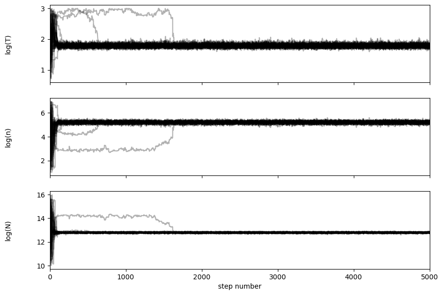
It seems that the walkers soon get converged after tens of steps. We can see how long it takes for the chains to “forget” where they start (this is the so-called autocorrelation time or the “burnt-in” time):

tau = sampler.get_autocorr_time()
print(tau)

[48.27226482 51.14776226 31.51566688]

That means the “burnt-in” time is ~30-50 steps. emcee will return an error if tau is larger than nwalkers/50, which means that the fitting has not probably converged yet, and you need to increase walkers or make some other modifications.

The results

Let’s discard the initial 200 steps (should be several times tau), thin by about 10 steps, and flatten the chain so that we have a flat list of samples:

flat_samples = sampler.get_chain(discard=200, thin=10, flat=True)
print(flat_samples.shape)

(19200, 3)

We can see the corner plot with:

fig = corner.corner(flat_samples, labels=labels, 
    truths = [np.percentile(flat_samples[:,0],50), np.percentile(flat_samples[:,1],50), np.percentile(flat_samples[:,2],50)]
)

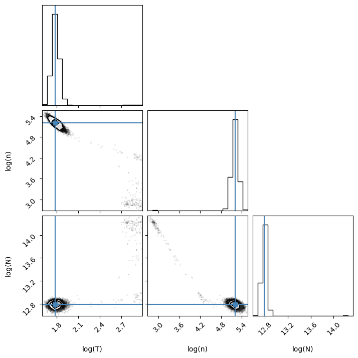
Seems good! The points cluster at the best-fit values, which are delineated with blue lines. To obtain the best-fit values and the 1$\sigma$ ranges, we can simply run:

for i in range(ndim):
    mcmc = np.percentile(flat_samples[:, i], [16, 50, 84])
    print(mcmc)

[1.73293549 1.78028829 1.83438747]
[5.11362719 5.20639793 5.29617062]
[12.75070224 12.78918629 12.82724839]

This means thae the best-fit values are 1.78, 5.21 and 12.79, and the $1\sigma$ ranges are [1.73, 1.83], [5.11, 5.30] and [12.75, 12.83] for log_T, log_n and log_N, respectively. This is roughly consistent with the values found by Podio et al. (2014).

Notes

I was trying to fit the four inversion lines of p-NH₃, i.e. (1,1), (2,2), (4,4) and (5,5), when I first want to use MCMC for RADEX. However, I got into trouble. The key is that, the inversion lines of NH₃ are a good thermometer of molecular gas, but they are insensitive to the gas density (See the introduction part of Lebrón et al. (2011)). Similar non-LTE analysis also failed to constrained the gas density even with up to 6 transitions of NH₃ (e.g. Feng et al. (2022)). Such phenomenon has also been found with transitions of CO (Dell’Ova tl al. 2020). In this article, the authors found that when the density is higher than 10⁴ cm^-3, the chi-square does not change significantly. This is probably because the critical densities of CO lines are rather low, so the lines will be thermalized at high densities, which leads to the weak dependance of integrated intensity on density.
Here is a possible solution to this problem. If you are sure that the density in you target cloud is much higher than the critical density of NH₃ or CO, you can leave the gas density as a constant instead of a variable. You would not expect (however, you may need to check that) you fitting results to vary a lot with different densities, say, 10⁴, 10⁵, and 10⁶ cm^-3. The uncertainty brought by unknown density is supposed to be lower than that brought by data reduction.